True peak: why samples below zero can still clip

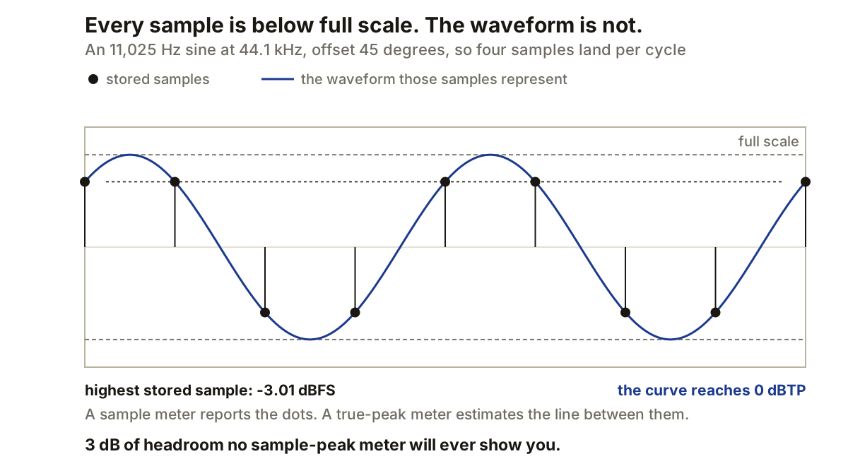
A sample-peak meter checks the highest stored sample value. A true-peak meter estimates the continuous waveform those samples represent. The two readings can differ, because the reconstructed waveform may reach its maximum between sample positions.

That gap matters near digital full scale. A file can contain no sample above 0 dBFS and still produce a reconstructed peak above that level during conversion, filtering or later encoding.

Samples are points, not the complete curve

At 48 kHz the system stores 48,000 samples per second, so the time between adjacent samples is 20.833 microseconds. At 44.1 kHz it is 22.676 microseconds. The stored values describe the waveform at those instants, and a reconstruction filter uses the sequence to recreate the continuous signal between them.

A sample-peak meter only needs to find the largest absolute number in the file. That calculation says nothing about the curve between samples. Adjacent values can sit below the ceiling while the reconstructed curve joining them rises higher.

A four-sample example exposes the difference

Use a 44.1 kHz session and generate a sine at one quarter of the sample rate, which is 11,025 Hz. At that frequency consecutive samples are 90 degrees apart, because four samples complete one cycle. Give the sine a 45 degree phase offset and its stored sequence becomes:

+0.707, +0.707, -0.707, -0.707

20 * log10(0.707) = -3.01 dBFS

The continuous sine still reaches plus and minus one between those stored points. Its reconstructed peak is therefore 0 dBTP even though the sample meter stops at -3.01 dBFS. Three decibels of headroom that no sample-peak meter will ever report.

This is a constructed worst-position example rather than a typical music signal. It proves the mechanism without relying on a particular limiter or converter.

True-peak meters estimate the missing curve

A true-peak meter oversamples the signal. It runs the samples through an interpolation filter and evaluates additional points between the originals, which gives a closer estimate of the reconstructed waveform.

The ITU true-peak algorithm specifies 4x oversampling for a 48 kHz input, producing a 192 kHz measurement stream. Four times as many sample positions reduce the spacing from 20.833 microseconds to 5.208. For a 96 kHz input the document states that 2x oversampling is sufficient to reach the same 192 kHz measurement rate.

Oversampling does not reveal a hidden set of samples stored in the file. The meter calculates estimates from the existing sequence and its reconstruction filter, so different meters can report slightly different maxima if their filters or oversampling factors differ.

The unit dBTP identifies this reconstructed-peak estimate. dBFS normally refers to sample values relative to digital full scale. A reading of +0.4 dBTP means the estimated continuous waveform reaches 0.4 dB above full scale, even if no stored sample crosses 0 dBFS.

Processing can create a new peak

Peak position depends on phase as well as level. Equalisation and sample-rate conversion use filters that rebuild the waveform, and the ITU specification notes that filtering and bit-rate reduction can increase peak level.

This is why checking only the limiter input is insufficient. A limiter may hold every sample below its ceiling, then a later resampler or encoder may produce a different reconstructed maximum. The delivered file needs its own measurement.

Lossy coding deserves particular attention, because the decoded waveform is not sample-for-sample identical to the source. Keep the unencoded master, create the required delivery file from it, and measure the decoded result. If it exceeds the intended ceiling, lower the level upstream and encode again.

True-peak limiting changes the detector

A sample limiter reacts to stored samples. A true-peak limiter oversamples its detection path so gain reduction can respond to estimated intersample maxima.

That can produce more gain reduction than sample-peak limiting at the same numeric ceiling, because the limiter is controlling values the sample detector never reports. Switching true-peak mode on after setting the rest of a master can therefore change both peak reduction and output level.

Place the final true-peak limiter after signal-changing master processing. If sample-rate conversion happens during export, analyse the rendered file afterwards, because the conversion occurs beyond the plugin chain. A true-peak limiter cannot account for every later operation: it controls the signal at its own output according to its own detector.

Measure the file that will leave the room

Use a sample meter while mixing to catch ordinary overloads. Add true-peak analysis when the signal approaches the ceiling or when preparing a delivery file.

Render the target sample rate and bit depth, then open that file in an offline analyser and compare sample peak with true peak for each channel. The difference between them is the intersample margin for that render.

Do not normalise or adjust gain after this check. Any level change creates a new file that needs another measurement, and the same applies after sample-rate conversion or encoding.

For troubleshooting, keep the process short: measure the unprocessed file, the output of the final limiter, the rendered delivery file and any encoded derivative. The first stage where true peak rises identifies the operation that needs more headroom.

Producer’s note

You can build the example above in a minute and watch both meters disagree.

At 44.1 kHz, generate an 11,025 Hz sine with a peak amplitude of one and a 45 degree phase offset. Mute the monitors first. The stored samples should peak near 0.707, which is -3.01 dBFS, while a true-peak meter should approach 0 dBTP.

If both meters show about -3 dB, confirm that true-peak analysis is enabled and inspect the generated samples. A different starting phase changes the result, which is the whole point: the same tone at the same level can hide a very different amount of intersample headroom depending on where the samples happen to land.